Inside Robot Data Pipelines: Filtering, Autolabeling, and Training Processors

Introduction

Modern vision-language models attach a pretrained vision encoder to a pretrained LLM backbone via a lightweight adapter, then train the combination through a staged curriculum—typically adapter-only alignment first, to map visual features into the LLM's embedding space without disturbing its weights, followed by broader fine-tuning once that mapping is established. The explicit goal at every stage is to preserve as much of the LLM's pretrained language understanding as possible while grafting on a new modality. Under that constraint, data curation, diversity, and quality end up mattering far more than sheer dataset size.

I think about robotics training the same way. There is no internet-scale corpus of robot trajectories to fall back on, so preserving pretrained knowledge and choosing carefully what new data you add to it is not optional—it's the whole game. Data diversity is everything. Knowing how to curate a small, high-quality, mode-covering dataset is consequently one of the highest-leverage skills in building a robot foundation model, often mattering more than raw scale.

In this post, I'll gradually introduce all of the core system components and architectural patterns that make up a modern, production-grade robot data processing pipeline. In particular, I'll be doing an under-the-hood breakdown of how raw, stored robot datasets get cleaned, enriched, and dynamically transformed for policy training: offline quality filtering and curation, dataset mixing and action-space harmonization, model-assisted autolabeling, and the online processors that sit at the dataloader boundary.

This post is the third in a series. Inside ROS 2 covered the real-time communication fabric that streams sensor payloads on-robot. Inside Robot Data Storage covered how those streams become durable, indexed MCAP logs and chunked, sharded Zarr datasets. This post bridges the gap between stored arrays and a converged model: how a raw, heterogeneous corpus becomes a clean, annotated, high-yield dataset that a foundation model or policy can actually learn from.

Like the rest of the series, this one follows an inverse-pyramid approach—starting broad with pipeline-level mechanics and the shape of the problem, then layering in system implementations, data structures, and concrete algorithms as we go, so you come away with an accurate mental model of the full pipeline before getting lost in any one stage of it.

Structure

1. The Problem: The garbage-in, garbage-out bottleneck—why physical robot data is noisy, redundant, unannotated, and expensive to train on blindly.
2. Filtering & Curation (Offline Ingest): Kinematic and dynamic sanity checks, sensor health assertions, contact/grasp validation, trajectory deduplication and diversity sampling, operator/source quality tracking, instruction-action alignment filtering, upsampling, and held-out split construction.
3. Dataset Mixing & Action-Space Harmonization: Co-training ratios across heterogeneous embodiments and sources, and the action-space harmonization required before an episode is eligible to be mixed in at all.
4. Autolabeling & Dataset Enrichment: Leveraging foundation models—VLM captioning, instruction paraphrasing, success/failure scoring, and confidence-cascaded labeling—to auto-annotate unlabelled teleoperation streams, plus a note on egocentric human-video pipelines for cross-embodiment data.
5. Online Training Processors: History-buffer assembly, action chunking and relative encoding, augmentation, conditioning dropout, proprioceptive noise injection, and curriculum-weighted sampling at the dataloader boundary.
6. Scale & Orchestration: Distributing filtering and autolabeling across frameworks like Ray and Spark, scheduling cloud-API vs. on-prem autolabeling against their real throughput ceilings, incremental processing for continuously-arriving fleet data, and the dataset versioning and lineage tracking needed to reconstruct exactly what a model trained on.

Notes & Assumptions

• Target Audience: Machine learning engineers, robotics researchers, and data infrastructure engineers who want to design robust, automated data refinement pipelines for robot foundation models and VLA architectures.
• Scope Boundary: This post assumes your data already lives in a chunked, queryable format—the MCAP/Zarr layout established in Inside Robot Data Storage, indexed via the manifest system established in that post, which the filtering and mixing covered here build directly on top of. Our entry point is that raw Zarr/MCAP boundary; our exit point is the tensor entering the model's forward() pass. Everything upstream of raw storage (ROS 2, DDS, rosbag2) and everything downstream of a trained checkpoint (policy serving, deployment) is out of scope here. This post assumes familiarity with the featurization and indexing layers from Inside Robot Data Storage—in particular, the ETL boundary between MCAP logs and Zarr arrays.
• A Note on Philosophy: Unlike the previous two posts, which were largely mechanical (how DDS discovery works, how Zarr chunks map to shards) and walked through real implementation code, a meaningful fraction of this post is judgment calls rather than fixed procedure—how aggressively to filter, how to weight a mixture, what counts as a good caption—and it stays at the level of architecture and tradeoffs rather than code. Where the field has a clear gold standard, I'll say so directly; where it's still an open, actively-debated design decision, I'll say that too.

The Problem: The Garbage-In, Garbage-Out Bottleneck

Everything in the previous post assumed that once an episode was durably captured and featurized into Zarr, the hard part was over. It isn't. A featurized corpus is complete in the sense that every array is populated and every chunk decompresses cleanly—but "complete" and "trainable" are different properties, and robot data collected from human teleoperation, scripted routines, or autonomous fleet execution fails to be the second one in ways that are easy to miss if you never look past the array shapes.

Unlike web-scale text or clean image-text pairs scraped from the internet, physical robot logs suffer from distinct real-world failure modes:

• Dead Time & Teleop Stalls: Even well-run teleoperation setups accumulate a meaningful share of idle time in the raw log—the operator standing still, readjusting VR controllers, or resetting the physical environment between attempts. None of this is corrupted data—every frame is valid, timestamped, and correctly featurized—but a policy trained on it learns that doing nothing is a common and rewarded action.
• Hardware Anomalies: Thermal throttling causing dropped camera frames, encoder slippage, ROS 2 topic timestamp drift, and camera lens smudges. These are the failure modes the previous post's featurization step silently assumes away when it resamples onto a common timeline—a dropped frame doesn't fail the ETL job, it just gets interpolated into something that looks plausible.
• Missing Semantic Metadata: Raw motor logs contain exact joint angles at high precision, but nothing about intent. No language instruction ("pick up the red mug"), no task boundaries, no success or failure signal. A Zarr array of joint states and image tensors is, on its own, semantically empty.
• Imbalanced Trajectory Distributions: A small set of common trajectories and paths—simple pick-and-place motions, in particular—tend to dominate most collected corpora by sheer frequency, which skews the trained distribution toward whatever was easiest or fastest to collect repeatedly. The direct cost is on the other end of that imbalance: less-traveled trajectories—recovery behaviors, contact-rich manipulation, rare edge cases—end up under-covered relative to how often they'll actually matter at deployment, which shows up downstream as poor recoverability and narrow mode coverage rather than as a policy that's simply "worse" in some diffuse sense.

Naively feeding raw physical logs directly into policy training wastes compute on frames that carry little signal, and—more fundamentally—a policy trained this way inherits whatever biases are present in the underlying data distribution, rather than the intended task distribution. Idle time is one common example: if a large share of the corpus is dead time, the policy has no reason to treat inaction as anything other than a normal, learned response, which can surface at inference as hesitation or stalling. A dropped frame silently interpolated into something plausible is a subtler version of the same problem: the policy is trained against a signal that was never actually observed, and has no way to know the difference. But the underlying dynamic is general, not particular to idleness or corrupted frames—it applies to any artifact the log overrepresents, whatever form that artifact takes.

The instinct this creates is to over-correct toward minimalism—strip everything down to just the frames that "matter." That instinct is usually wrong. Data is the foundational material a policy learns from, so the safer failure mode is the opposite of that instinct: label as much as you can.

Episode score, duration, success/failure, captioning, operator or policy ID, embodiment, station—every one of these becomes a conditioning signal that partitions the data manifold into distinguishable sub-modes rather than one undifferentiated blob. That partitioning is what makes guidance possible: if the model has learned the difference between, say, a slow success and a fast one, those become separable manifolds it can be steered between at inference time—conditioning on "fast" pulls the policy toward that subpartition specifically, rather than the model only ever producing whatever the average of both looks like. The same partitioning is what makes filtering, diversity curation, and interpretability possible after the fact, none of which exist if the corpus is unlabeled to begin with.

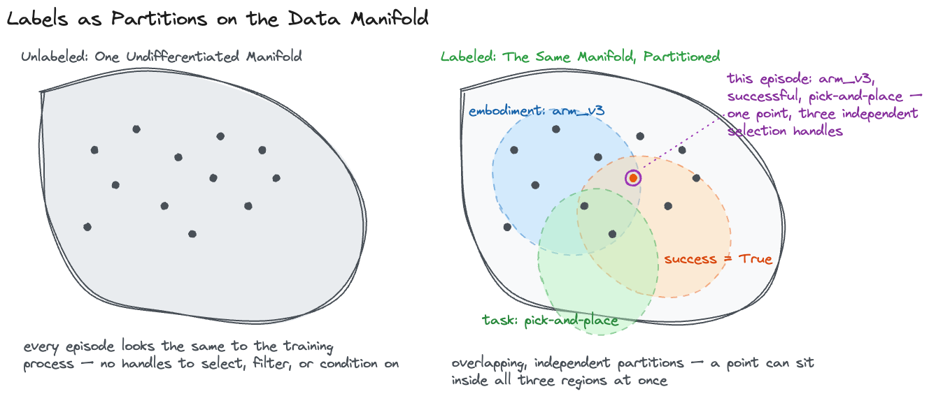
You can always choose to ignore a label at training time. You can't retroactively add one without a full re-labeling pass.

The rest of this post is organized around that asymmetry: first the offline filtering stage that decides what's in the corpus and what gets thrown out, then the mixing stage that decides what target mixture the corpus should be trained toward, then the autolabeling stage that decides what semantic signal gets attached to what survives, and finally the online-processing stage that reshapes all of it, on the fly, into what a training step actually consumes.

The Data Refinement Pipeline

A raw, uncurated Zarr/MCAP corpus becomes a high-yield training corpus by passing through four stages, all of which read from and write back to the manifest layer established in the previous post—so "processing" a corpus is less a series of file conversions and more a series of columns and flags accumulating on top of the same indexed episodes. One thing has to happen before any of it: action-space harmonization, reconciling embodiment-specific action representations so an episode is even eligible to enter the manifest. This has to come first because nothing downstream is meaningful without it—kinematic sanity checks, for instance, don't mean anything across embodiments whose action spaces haven't been reconciled yet.

• Raw Storage (MCAP / Zarr) → Action-Space Harmonization
• Stage 1: Offline Filtering & Cleaning — deterministic and learned quality gates, writing pass/fail flags and quality scores back to the manifest
• Stage 2: Dataset Mixing — corpus-wide mixture weights, written to and read from the manifest at sampling time
• Stage 3: Autolabeling & Enrichment — foundation-model annotation, writing captions and confidence scores back to the manifest and/or as new Zarr arrays
• Stage 4: Online Training Processors — per-batch, per-epoch transforms applied inside the dataloader
• Policy Forward Pass

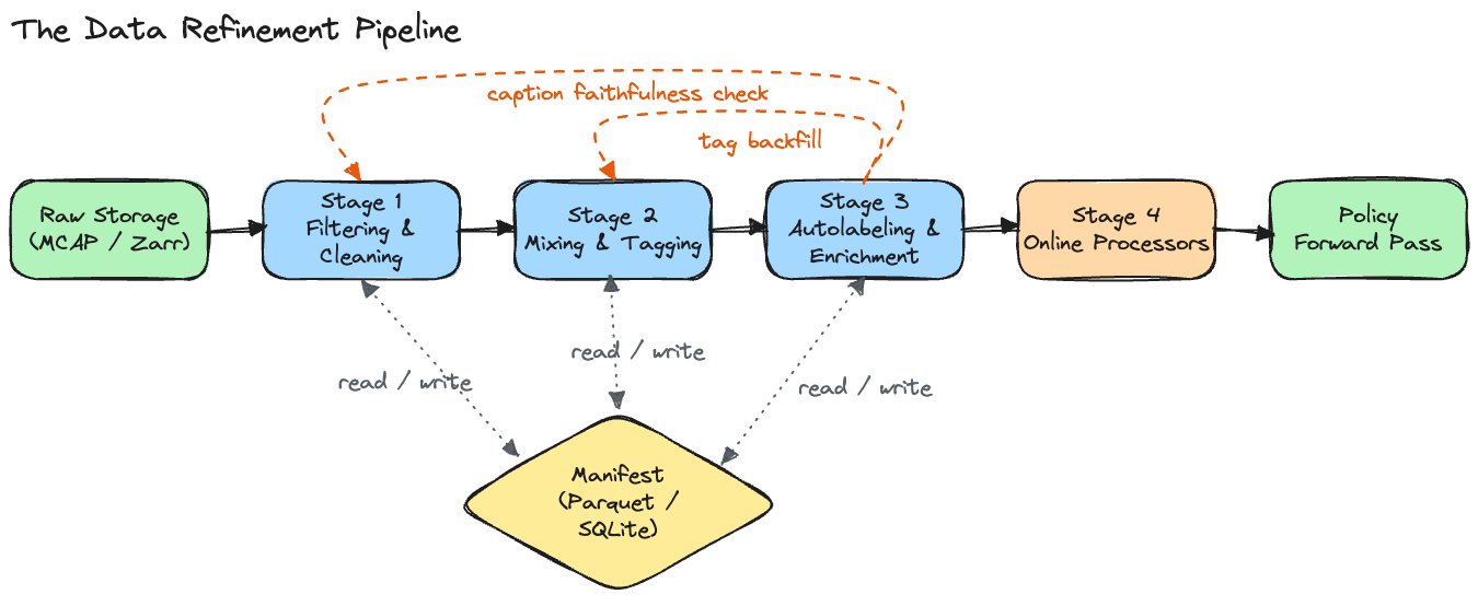
This ordering matches how the post is structured, but it's not a strict dependency chain where each stage fully finishes before the next begins. It's closer to "the order in which each stage's output usually gets used downstream," and there are two real feedback loops that cut across it:

• Autolabeling feeds back into filtering. Once a caption exists, it gets checked against the trajectory it's supposed to describe. If a caption doesn't hold up, that episode gets flagged and sent back through filtering—so labeling can retroactively change whether an earlier episode is considered clean.
• Mixture ratios depend on results you don't have yet. The "right" mix of data sources isn't something you can calculate up front—it only becomes clear after training candidate mixtures and checking them against held-out data. That means tuning the mixture is really an outer loop wrapped around the whole pipeline, not a decision made once and locked in.

None of this breaks the four-stage mental model—it's still the right way to think about what each stage does. It just means a "stage" is a category of work, not a single station every episode passes through exactly once on a one-way trip.

Offline Filtering & Curation: Cleaning Raw Logs

Before running expensive neural network labelers or committing GPU-hours to a training job, it's worth being precise about what this stage is actually catching. Raw logs aren't full of subtle problems—they're full of obvious ones: a joint commanded past what the actuator can physically do, a camera frame that's pure sensor noise, ten seconds where nothing in the scene moves at all. None of these need a model to catch. They need a rule. The filters in this section are a battery of fast, mostly-deterministic heuristic checks—not because the problems they catch are unsophisticated, but because sophistication would be wasted on problems this cheap to detect. The goal isn't semantic understanding. It's triage: strip out what a simple rule already knows is broken, so the expensive stages downstream only ever spend their compute on logs that actually deserve it.

The checks that follow are a representative sample, not an exhaustive one—there are many more filters and heuristics in production use than any single post could cover, and new ones get written the moment a new failure mode shows up in the data. What matters is the pattern each one follows, not the specific list.

Kinematic & Dynamic Sanity Checks

These checks share a single question: is the motion itself physically plausible, independent of what the robot was supposed to be doing? A joint trajectory can be perfectly timestamped and still be nonsense—a glitch, a dropout, a command no real actuator would produce.

• Velocity and Acceleration Caps: Flagging trajectories where joint accelerations exceed physical actuator limits ($\ddot{q} > \ddot{q}_{\max}$), which often indicates encoder dropouts or teleoperator glitches rather than genuine robot motion (though a genuine physical event—a collision, a dropped payload—can occasionally produce the same signature, so this flag is a strong prior for triage, not a certain diagnosis).
• Singularities & Self-Collision Checks: Filtering frames where arm kinematics approach gimbal lock or internal self-collision boundaries—both produce erratic, high-magnitude joint commands that are kinematically valid but not representative of intended behavior.
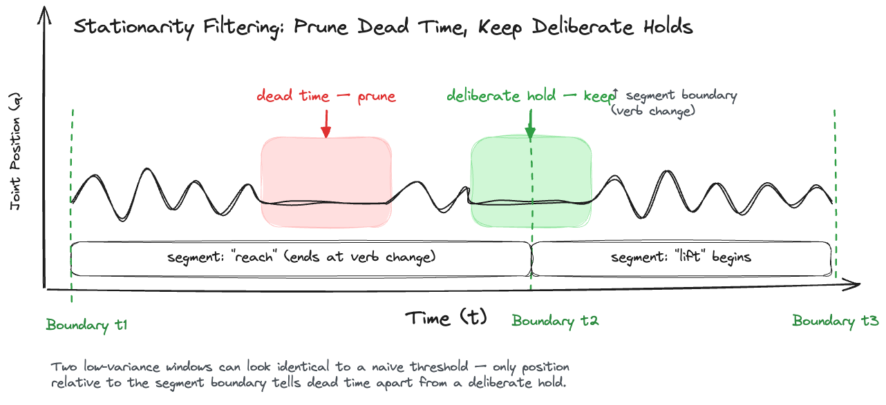
• Stationarity & Motion Thresholding: Detecting long stretches of static joint positions using sliding-window variance:

Pruning static frames prevents a policy from learning idle, non-responsive behavior as a common mode. This is one of the highest-yield filters against the dead-time problem discussed earlier.

Sensor Health Assertions

Kinematic checks ask whether the robot's own motion makes sense. This section asks the same question about the cameras recording it—a perfectly valid trajectory is worthless if the footage of it is corrupted, misaligned, or silently degraded.

• Timestamp Jitter & Frame Drop Auditing: Validating that image topic timestamps remain within a strict $\Delta t$ window ($33\text{ ms} \pm 5\text{ ms}$ for 30 Hz feeds). Dropped frames are either forward-filled or the entire episode is quarantined, depending on drop severity.
• Image Quality Checks: Blur detection via Laplacian variance—convolving each frame with a Laplacian (second-derivative) kernel and thresholding on the variance of the response, since a sharp image has strong edges everywhere and therefore high-variance second derivatives, while a blurred one doesn't—along with over/under-exposure clipping and black-frame detection.
• Multi-View Consistency Checks: Single-stream checks catch a dead camera; they don't catch two live cameras that have silently drifted out of sync, or a second view that's occluded while the primary view looks fine. For multi-camera rigs, cross-view consistency—verifying that all views are timestamp-aligned and none has silently degraded—is a distinct check from per-stream health, and one that's easy to skip if you only ever look at one camera during a debugging pass.

Contact & Grasp-Based Filtering

Kinematic and image-level checks say nothing about whether a manipulation actually happened. A trajectory can be smooth, in-frame, and correctly timestamped while still representing a failed or phantom grasp—and that's a distinct failure mode worth its own filter class:

• Force-Torque Contact Validation: Flagging episodes where a "pick" is claimed (via caption or heuristic) but the F/T sensor shows no contact spike at the expected timestep—a strong signal of a missed or slipped grasp that other checks won't surface.
• Gripper-State Transition Validation: Confirming the gripper actually closes past a meaningful threshold when a grasp is claimed, rather than hovering near the open position for the full "grasp" segment.

These checks are cheap relative to autolabeling and catch a class of error that captioning models frequently miss, since a VLM judging success from RGB frames alone can be fooled by a visually plausible but physically failed grasp.

Diversity Sampling & Trajectory Deduplication

The checks in the above filters are pass/fail gates—they decide whether an individual episode is valid. This section is a different kind of filtering: even a corpus made entirely of valid episodes can be badly shaped, if it's dominated by whichever task, environment, or trajectory happened to get collected the most. The goal here isn't removing bad episodes, it's actively shaping which valid episodes end up represented, and how often. Deduplication is one tool in service of that goal, not the goal itself.

• Caption Clustering and Sampling: Run a POS-tagger (or lightweight LLM) to extract noun-phrases and verbs from segment captions. Perform uniform sampling across (verb, direct-object) buckets. This ensures episodes are diverse in object interactions and interaction types, rather than dominated by whatever task happened to be collected most.
• Environment Clustering: Use an embedding model to create scene embeddings and sample uniformly across environments, rather than letting whichever station collected the most hours dominate the corpus.
• Trajectory Clustering: Using dynamic time warping (DTW) over end-effector poses to cluster similar trajectories and downsample duplicate successful runs—this is where deduplication proper comes in, as the mechanism for trimming an overrepresented cluster back down once sampling has identified it.

Quantitative Coverage Metrics: Two Axes, Not One. "Diversity is king" is easy to say and hard to measure, and one reason it's hard to measure is that "diversity" is usually treated as a single number when it's really two independent properties of the corpus:

• Breadth: how many distinct buckets exist in the corpus at all—how many (verb, object) pairs, how many environments, how many trajectory clusters are represented, regardless of how much data sits in each one.
• Evenness: given the buckets that do exist, how uniformly the corpus is spread across them—whether episodes cluster overwhelmingly into a handful of buckets or are actually distributed across the full breadth the corpus claims to have.

These pull apart in practice more often than the single word "diversity" suggests. A corpus can have excellent breadth—hundreds of distinct verb/object combinations, dozens of environments—while still being badly uneven, with 80% of episodes concentrated in "pick up cup" across three of those environments and the remaining breadth represented by a handful of episodes each. Conversely, a corpus can be nearly perfectly even across a narrow breadth—uniformly sampled, but only ever pick-and-place in a single room—and still fail to cover the task space a deployed policy needs. Neither failure mode shows up if you only track one number.

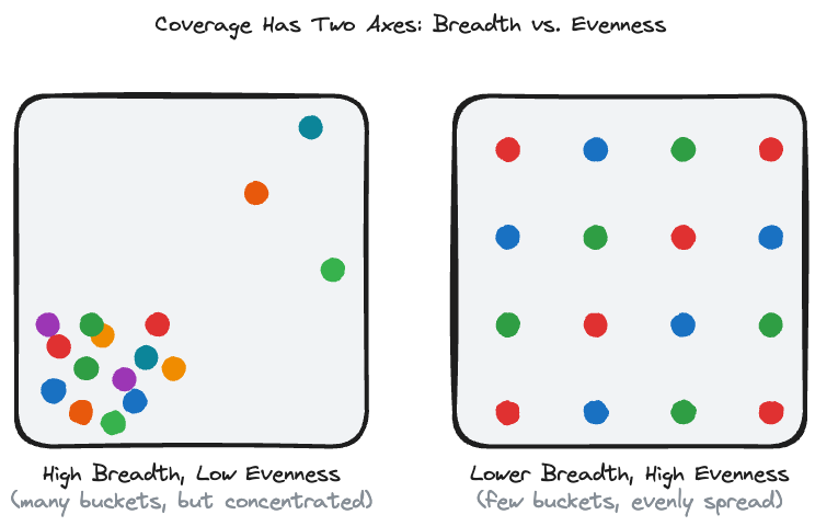
Concretely, this argues for reporting both: an entropy or histogram-based evenness score, and a raw count of distinct buckets (from embedding-space clustering or the caption-derived verb/object buckets above) as a separate breadth score. A corpus that "feels diverse" and a corpus that scores well on both axes are not always the same corpus—and a corpus that scores well on only one of them is a specific, nameable kind of imbalance rather than a vague shortfall, which makes it something the upsampling pass covered next can actually target: low breadth calls for collecting or mixing in new buckets entirely, while low evenness calls for upsampling the underrepresented buckets you already have.

Upsampling

Filtering removes; upsampling redistributes. Not all data is created equally, and (once again) diversity is king—ideally your dataset covers a broad enough span of states that if the robot were to reach any theoretical state, there is training signal showing how to recover from it. This is what makes DAgger (Dataset Aggregation)—where an operator corrects a failing rollout mid-trajectory—particularly high-value data: it directly provides error-correction signal that on-policy successful demonstrations never generate on their own. Balancing diversity isn't limited to scene and object coverage; it extends to error correction, near-failure recovery, and outright failure, all of which are typically underrepresented relative to how often they'll matter at inference time.

Operator & Source Quality Tracking

Everything above—deduplication, upsampling—shapes which valid episodes get emphasized and how often. This section asks a question that's logically prior to all of that: is a given source of episodes any good in the first place?

Teleoperators, scripted collection policies, and simulation generators vary meaningfully in trajectory quality, and that variance is worth tracking explicitly: per-operator or per-source success rate, motion smoothness, and intervention frequency, stored as manifest-level metadata and used either as a hard filter (dropping a chronically low-quality source) or a soft signal feeding into sample weighting during training.

Instruction–Action Alignment Filtering

This is the one filter that can only run after autolabeling has produced a caption, which is why the pipeline described earlier isn't strictly one-directional. Once an episode has a generated instruction, a natural question is whether that instruction actually describes what happened—and it's worth being precise about what "agreement" means here, because a coarse gist-level check misses a specific and common failure mode.

The naive version of this filter asks a VLM-as-verifier a single holistic question—"does this caption match this video?"—and thresholds on the response. The problem is that a caption can be broadly right and still wrong in exactly the way that matters: "pick up the cup and place it in the sink" can score as a plausible match against a video where the robot picked up the cup, hesitated, set it back down, and then placed a different object in the sink—because the overall gist (something was picked up, something ended up in the sink) is superficially consistent, even though the actual sequence of sub-goals doesn't match at all.

A Sharper Version: Alignment as Sequence Matching, Not Gist Matching. Because an episode decomposes into segments bounded by verb changes—a concept covered in more detail in the autolabeling section below—alignment checking can be reframed as a structured problem instead of a fuzzy similarity judgment: extract the sequence of verbs a verifier independently derives from the video (reach → lift → carry → place), and compare it against the sequence of verbs implied by the caption's own segmentation, rather than comparing the two as unstructured blobs of text.

This turns "does the caption match" into something closer to a sequence-alignment problem—effectively an edit distance over verb sequences, where insertions, deletions, or substitutions in the verifier's sequence relative to the caption's sequence are countable, specific evidence of a mismatch, rather than a single opaque similarity score. An episode where the sequences align exactly is a strong pass; one where a full sub-goal is missing or substituted (the "hesitated and set it back down" case above) fails in a way that's actually visible in the comparison, rather than washed out by a holistic score that only looks at start and end state.

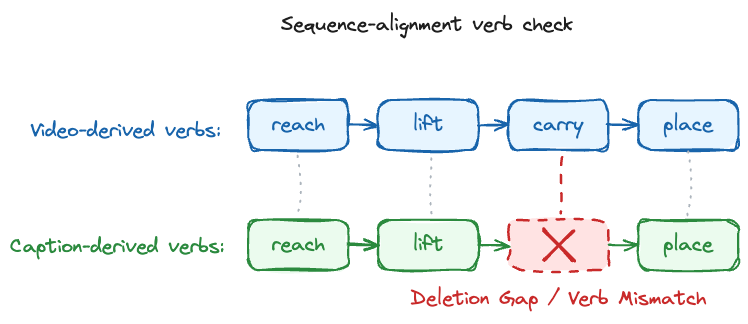
This closes the loop between filtering and labeling in a more rigorous way than a single-question verifier can: bad labels are a data quality problem, and checking them at the same segment granularity that produced them in the first place is a more faithful test than checking them against a coarser question than the one that generated them.

Held-Out & Evaluation Split Construction

Every filtering and upsampling decision above is made in service of a training split—but the same corpus has to yield a held-out set that actually tests what you care about, and that's easy to get wrong silently. A few failure modes worth naming explicitly:

• Leakage: the same station, operator, or physical object instance appearing in both train and eval inflates apparent performance without testing generalization.
• Wrong axis of generalization: a random episode-level split tests very little if every episode shares the same three scenes—scene-held-out, task-held-out, and object-held-out splits each test a different capability, and conflating them gives an eval number that doesn't mean what you think it means.
• Stratification: an eval set should be deliberately stratified along whichever axis is under test, not just randomly sampled and hoped to be representative.

Get this wrong and every downstream decision in this post—which filters to loosen, how to weight a mixture, whether an autolabeler upgrade helped—is being validated against a number that doesn't measure what it claims to.

Dataset Mixing & Action-Space Harmonization

Before getting into how a mixture ratio actually gets set, filtering and mixing are answering two different questions. Filtering asks something about one episode at a time: is this one any good? Mixing asks something about the whole corpus at once: a real kitchen and a simulated one, one robot's gripper and a structurally different robot's gripper, a teleoperated grasp and a human hand reaching for the same mug—how much of each should end up in the training set, and on what basis do you even compare them? That's a different kind of decision, made at a different layer than filtering, and it comes with its own prerequisite: two episodes can't be weighed against each other until their action spaces actually mean the same thing, which is why harmonization has to happen before a ratio can even be set.

Those examples weren't picked at random—they're the four axes that actually show up in practice when "combine multiple datasets" stops being an abstraction and becomes a real decision:

• Cross-lab / cross-robot: the same general task (pick-and-place) collected on different physical robots, with different sensor suites and control stacks.
• Sim vs. real: procedurally generated or simulated rollouts mixed alongside real fleet data, trading collection cost for a real-vs-synthetic distribution gap.
• Cross-embodiment: data from a structurally different robot (a different arm, a mobile base, a different gripper design) than the one being trained for—valuable specifically because it transfers shared visual and task structure even when the action space doesn't line up.
• Human embodiment: egocentric human video (discussed later in this post) sitting at the far end of the cross-embodiment axis—no robot at all at collection time, useful for exactly the same reason cross-embodiment robot data is, just with a harder retargeting problem attached to it.

Every one of these is, at the mixing layer, the same problem: decide a target proportion, and make sure what's being mixed is actually comparable once it's in the corpus. The next two subsections are that decision and that reconciliation, respectively.

Mixture Ratios / Co-Training Weights

Upsampling and mixing sound similar but answer different questions. Upsampling redistributes emphasis within a dataset—more of this trajectory, less of that one. Mixture weighting sets the target proportion between datasets that may differ in embodiment, sensor suite, collection method, or modality entirely: how much of the corpus is sim rather than real, cross-embodiment rather than native robot data, egocentric rather than teleoperated—the same four axes from a moment ago, now expressed as a question of volume rather than kind. Modern VLA training recipes—RT-X, Octo, OpenVLA, and $\pi_0$-style co-training pipelines—explicitly tune ratios like "40% single-arm manipulation, 25% mobile navigation, 20% bimanual, 15% simulation," rather than pooling every available episode uniformly and hoping the resulting distribution is reasonable.

In practice these ratios are rarely derived analytically. The dominant approach is empirical: train candidate mixtures at reduced scale, evaluate against the held-out splits discussed earlier, and adjust ratios based on which capability moved and which regressed. This is expensive relative to a single training run, but far cheaper than discovering a bad mixture only after a full-scale run completes.

Where this gets genuinely underspecified, though, is cross-embodiment and egocentric sources. "Use a more conservative ratio for these" is the standard advice, but conservative relative to what, exactly? A percentage on its own doesn't tell you how much risk you're taking on, because two sources at the same volume can carry very different amounts of transfer benefit and transfer risk depending on how far they sit from the deployment embodiment.

A Two-Axis Way to Think About It: Volume and Distance. It's worth treating a mixture ratio as governed by two separate numbers, not one:

• Volume: the familiar percentage of the corpus a source occupies.
• Distributional distance from deployment: how much the source's camera geometry, action space, gripper morphology, and control frequency actually diverge from the robot the policy will run on.

These are independent axes, and conflating them is exactly what makes "be more conservative" hard to act on. A cross-lab source collected on the same robot model, same gripper, same camera rig as your deployment target is low-distance—even if it's a large fraction of the corpus, it's a comparatively safe bet, because whatever it teaches the policy transfers close to directly. Egocentric human video, by contrast, is high-distance on every one of those axes at once—different sensor, no native action space, a hand instead of a gripper—so even a modest volume contribution is a much larger bet, because the policy has to bridge that whole distance through the retargeting pipeline discussed later before any of it is directly useful.

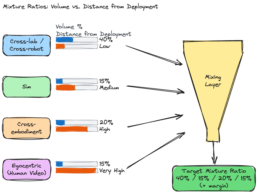
Concretely, that suggests a rough budget: a source's mixture weight should scale down as its distance from deployment goes up, and the two shouldn't be set independently. A 20% allocation might be perfectly reasonable for a low-distance cross-lab source and clearly too aggressive for a high-distance egocentric one, even though "20%" looks identical on a mixture-ratio spreadsheet. In practice this means tracking distance as its own attribute alongside the source itself—camera intrinsics match, action-space overlap, gripper-type match—rather than trusting volume percentage alone to communicate how much risk a given ratio is taking on.

Action-Space Harmonization

Before an episode from a new embodiment can even be a candidate for mixing, its action representation has to be reconciled against whatever the rest of the corpus uses. Different robots have different DOF, different gripper types, and sometimes fundamentally different control conventions (joint-space vs. end-effector-space commands). This is a gate at ingest time, not a training-time convenience—padding unused dimensions, masking embodiment-specific action slots, and normalizing units per-embodiment all have to happen before an episode is eligible to sit in the same manifest as episodes from a different robot. Get the harmonization scheme wrong and every downstream mixture ratio is mixing action spaces that don't actually mean the same thing.

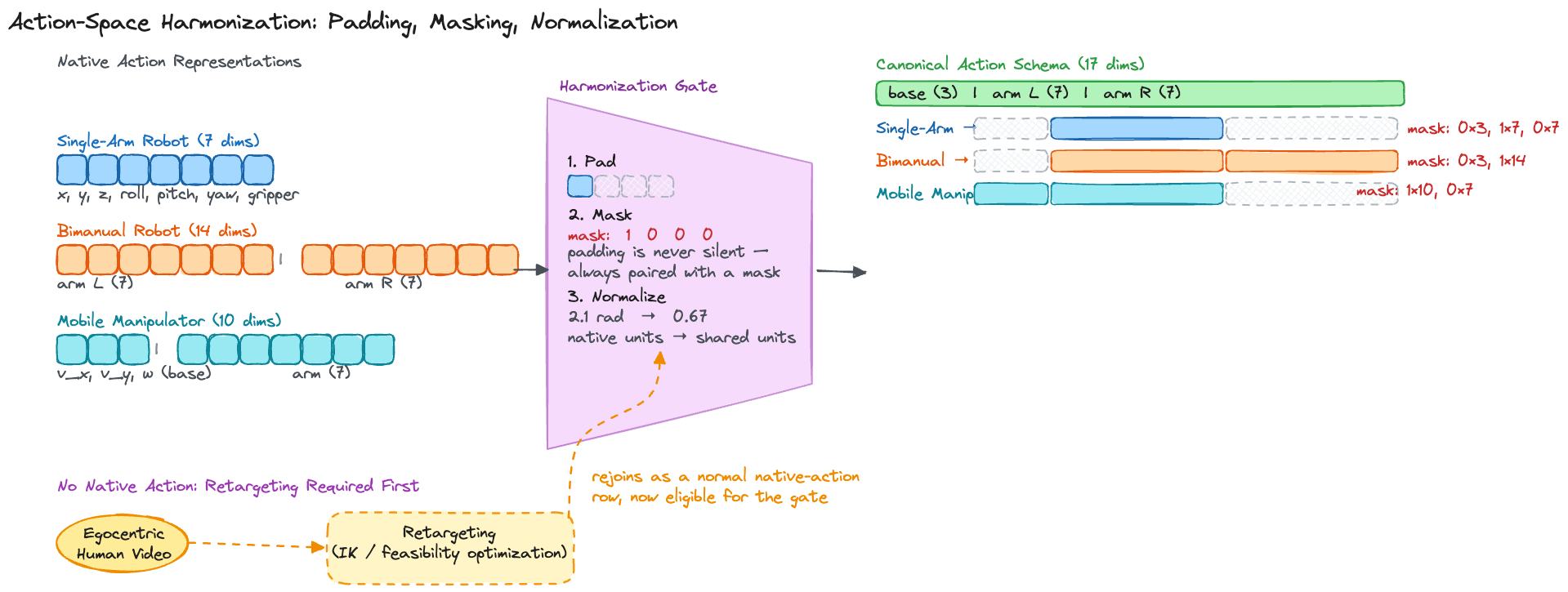
Cross-embodiment and human-video sources push this further than a same-embodiment mismatch does: there's no native robot action to harmonize until one has been produced. That's the retargeting problem discussed later—inverse kinematics and feasibility optimization mapping a human wrist trajectory into a robot-executable joint command—and it's worth flagging the dependency explicitly here: harmonization for those sources isn't a normalization step, it's downstream of an entire labeling pipeline substantial enough to be deferred to a future post.

Autolabeling & Dataset Enrichment

Raw robot logs contain low-level physical observations—joint angles, images, gripper state—but modern Vision-Language-Action (VLA) models need rich semantic labels on top of that: language instructions, sub-task boundaries, and success signal. Autolabeling uses pretrained foundation models offline, at corpus scale, to generate this signal without a human annotator touching every episode.

Trajectory Captioning & Instruction Generation

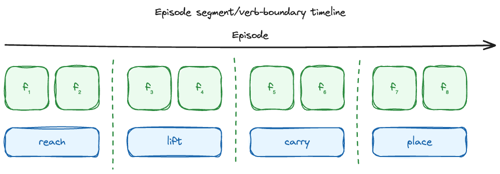
Before getting into how captioning is done, it's worth being precise about what's actually being labeled. An episode is a sequence of segments, each one the robot interacting with the environment in pursuit of some sub-goal—reaching, grasping, transporting, placing. A useful working definition of a segment boundary: it's the point in the episode where the verb changes. "Reach for the mug" and "lift the mug" are different segments; the transition between them is a segment boundary. Labeling an episode, then, is two coupled tasks—temporal segmentation (finding those transition/event boundaries) and captioning (describing what's happening within each resulting segment)—not a single caption applied to the whole trajectory.

Why this level of detail matters: caption quality isn't just a nice-to-have, it's directly connected to how well a pretrained VLM backbone adapts to the robotics domain in the first place. A sparse caption ("pick up spoon") is further from the kind of dense, descriptive language a VLM saw during its own pretraining than a detailed one ("pick up the metal spoon resting to the left of the bowl") is. The closer the caption distribution sits to the pretraining distribution, the less catastrophic forgetting the model suffers when it's adapted to robot data, and the better it retains the visual and semantic grounding that made it worth starting from a pretrained checkpoint at all. Sparse captions are the more common failure mode in practice, largely because they're the cheaper thing to produce—which is exactly why the density of an autolabeling method is worth treating as a first-class design criterion, not an afterthought.

Large Vision-Language Models (LLaVA, GPT-4o, Gemini Vision, and similar) can perform this segmentation-and-captioning task by processing keyframes sampled from an episode—start, middle, end, or a denser sample for longer trajectories—to output structured task descriptions: "Pick up the yellow sponge and place it in the sink."

The dense sub-goal annotation approach: segmenting long-horizon trajectories into sub-task milestones with timestamped boundaries, rather than one caption for the whole episode—i.e., actually doing the segmentation-plus-captioning task described above, rather than treating the episode as a single static scene to describe.

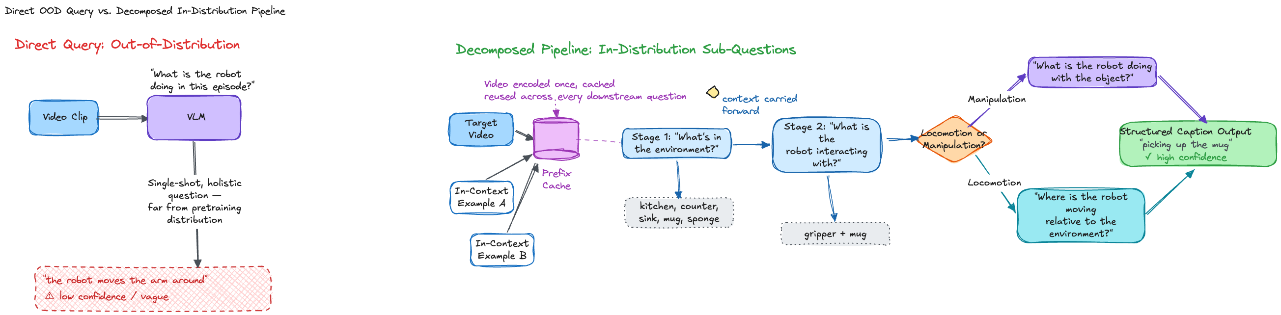
Most pretrained VLMs are out-of-distribution for this task straight out of the box—segmenting and captioning a multi-view robot episode looks very different from the single-image captioning or short-video-clip tasks these models were pretrained on, and out-of-the-box performance reflects that. Two approaches dominate in practice, borrowing heavily from techniques the video-generation and video-captioning communities already use for a structurally similar problem:

• Fine-tune on human-labeled data: have human labelers provide precise, high-quality temporal and text captioning across a set of highly diverse robot videos, then fine-tune an open-weight VLM on that set. This is the more reliable path, at the cost of an upfront human-labeling investment.
• Decompose the task into in-distribution sub-requests: rather than asking a VLM the OOD question directly ("what is the robot doing in this clip?"), a pipeline chains together a sequence of easier, more in-distribution questions that build up enough context to make the original question answerable—"what's in the environment?" → "what is the robot interacting with?" → "what is the robot doing?" This decomposition approach doesn't tend to work well as a from-scratch captioner for raw, unlabeled episodes—it's still fundamentally asking an OOD model to reason about an OOD task, just with better scaffolding. Where it does earn its keep is as a second-pass layer on top of captions that already exist: caption verification and confidence scoring (does this decomposed reasoning chain agree with the original caption?), and caption upsampling—densifying an existing sparse, accurate annotation into something closer to the detailed target described above, turning "pick up cup" into "pick up the yellow cup to the right of the bowl."

A Production Approach: Chunked Temporal-and-Text Captioning

To address the OOD gap identified above, a highly effective pattern is to constrain the input space to fixed-horizon video chunks, framing joint segmentation and captioning as a structured prediction task over bounded windows. It's built directly on the OOD diagnosis two paragraphs up: if the reason out-of-the-box captioning fails is that a full, arbitrary-length episode looks nothing like what a VLM saw during its own video-pretraining, the fix isn't better prompting or more scaffolding—it's changing the input so the task is no longer OOD in the first place.

The core idea is to fix the input to a short, bounded clip rather than an arbitrary-length episode, and train the model to jointly predict segmentation and captioning as structured output over that fixed window:

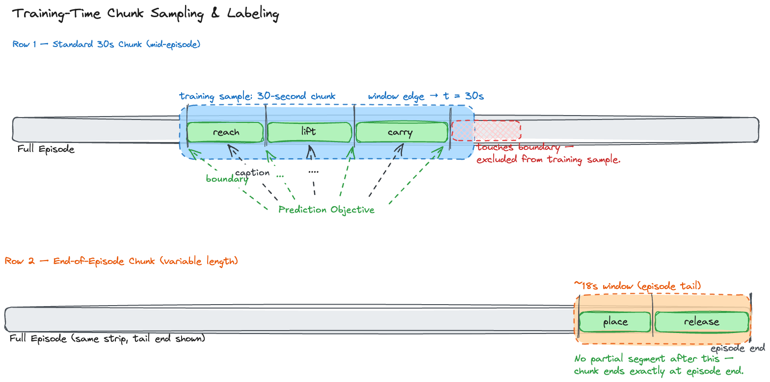
• Chunking: split each episode into fixed-size video chunks—120 frames at 4 fps, giving a 30-second clip per chunk, though the exact numbers are tunable to your domain and are far less important than the underlying principle. A 30-second clip is much closer in scale to the video-caption pairs a VLM saw at pretraining time than a multi-minute robot episode is, which is precisely what makes the task in-distribution again.
• Structured joint prediction: train the model to output, per chunk, a JSON object listing every segment fully contained within that chunk—its start/end frame and its caption—rather than a single caption for the whole clip. This directly operationalizes the segment-boundary definition from earlier in this section: the model isn't asked to describe a scene, it's asked to emit the same (boundary, caption) structure a human annotator would produce.
• The boundary-exclusion rule: segments that merely touch or cross the edge of the chunk are excluded from the label entirely, rather than included as partial or truncated. This is a small design choice that matters a great deal in practice—without it, the model is implicitly being trained to guess at segments it cannot actually see the end of, which teaches it to hallucinate plausible-sounding boundaries rather than genuinely detect them. Excluding edge-touching segments keeps every training label fully grounded in visible evidence.

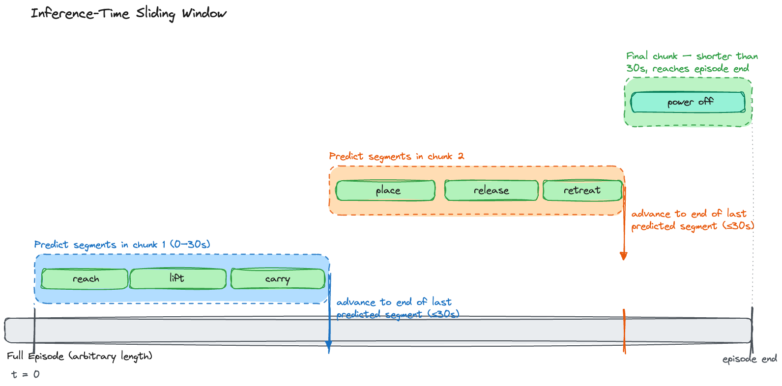
At inference time, this training scheme pairs with a simple sliding-window strategy to cover a full episode of arbitrary length: predict segments for the current chunk, then advance the window to the end of the last fully-predicted segment (not to a fixed stride), and repeat. Because partial, edge-touching segments were never part of the training distribution, the model reliably stops predicting cleanly at a true boundary near the edge of its window rather than mid-segment—which is exactly what makes "slide to the end of the last prediction" a stable strategy rather than one that drifts or double-counts segments over a long episode.

Instruction Paraphrasing & Language Augmentation

A single ground-truth instruction per episode is a narrower training target than it needs to be. Once a base caption exists, an LLM rewriting pass can generate several alternate phrasings of the same instruction—"pick up the mug" / "grab the cup" / "lift the yellow mug off the table"—without touching the underlying trajectory at all. This is purely an offline, corpus-time augmentation of the language label, distinct from the online conditioning dropout covered later in this post; it increases the diversity of language a policy sees for a fixed action, rather than varying whether language is present at all.

Success, Failure, and Quality Scoring

Earlier, this post named success/failure as one of the highest-value labels a corpus can carry, but didn't say how it gets produced. In practice, three mechanisms are common, roughly in order of cost:

• End-state VLM judging: passing the final frame(s) of an episode to a VLM with a judging prompt ("did the robot successfully place the object in the bowl?"). Cheap to stand up, but inherits whatever hallucination tendency the base VLM has—a visually plausible final frame can pass judgment even if the grasp along the way was a near-miss.
• Heuristic goal-region checks: geometric or state-based success criteria—object position within a target region, gripper state at episode end—when the task and success condition are well-defined enough to express as a rule. Cheaper and more reliable than a VLM judge where it applies, but brittle to task variety; it doesn't generalize to tasks nobody wrote a rule for.
• Learned reward/quality classifiers: a lightweight classifier trained on a small, human-labeled seed set of successes and failures, then run at corpus scale. This tends to outperform a zero-shot VLM judge once a seed set exists, at the cost of needing that seed set in the first place—typically bootstrapped from a few hundred to a few thousand human-reviewed episodes.

None of these are mutually exclusive—it's common to run a cheap heuristic where available and fall back to a VLM judge or learned classifier elsewhere, which is really a special case of the cascading pattern below.

There is a lot more to autolabeling than what's covered here, and plenty of approaches beyond these three that work well in practice—but this is enough to build on for the rest of the post.

Confidence-Aware & Cascaded Labeling

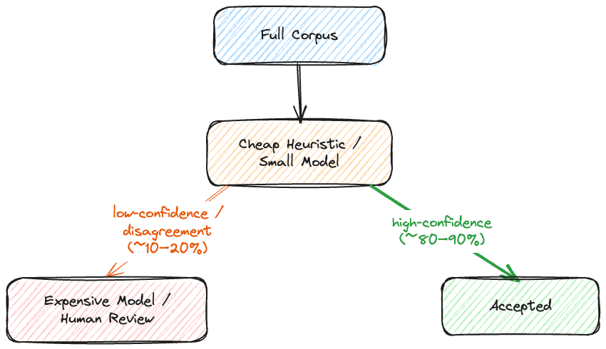
Every autolabeler above shares the same failure mode: it's occasionally, confidently wrong. Running the most capable (and most expensive) model on every episode is one way to minimize that risk, but it's rarely the most efficient one. A standard mitigation is a cascade:

• A cheap heuristic or small model runs first, over the full corpus.
• High-confidence outputs—cases where the cheap pass and any available cross-check agree—are accepted automatically.
• Low-confidence or disagreement cases are routed to a larger, more expensive model, or to a human review queue.

A Note on Learning from Human Video

Everything above autolabels episodes already collected on-robot. A distinct and increasingly common way to buy diversity without proportional robot-hours is egocentric human video—footage of a person performing a task, with no robot involved at collection time at all. The core difficulty is that human hand pose isn't robot action: getting from a hand trajectory to something trainable requires a retargeting pipeline—3D hand pose estimation, compression into a robot-relevant representation (often a virtual parallel-jaw gripper derived from thumb/index geometry), and inverse kinematics to map that representation onto an actual robot's joint space. That pipeline is substantial enough to be its own post; I'll leave it there for now.

Online Training Processors: Dynamic Training-Time Transformation

Everything up through autolabeling is offline: it runs once per episode, its output is written back to the manifest or the Zarr store, and every subsequent training run reads the same result. Online training processors are the opposite. They run inside the dataloader worker processes, once per sample per epoch, and produce nothing that gets written back to the corpus—their entire output is the tensor that goes into the model's forward() pass for this step, recomputed from scratch on the next one. (The curriculum sampler discussed later in this section is a partial exception: it reads persisted manifest data to decide what to sample, even though the transforms applied to what it samples are still transient.)

Observation Horizons & History Buffers

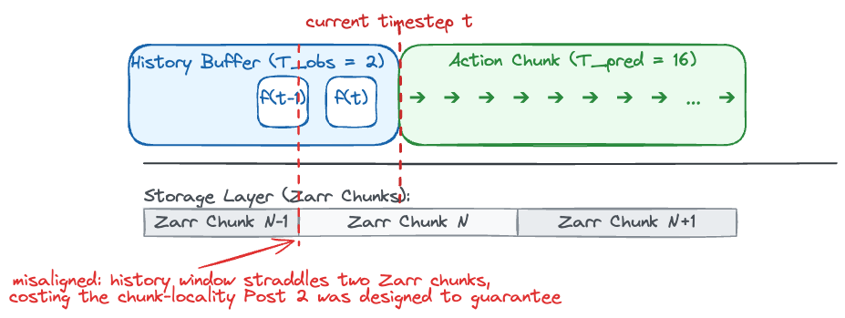
Assembling observation windows of length $T_{obs}$—for example, stacking the last 2 camera frames and joint states—to give the policy the temporal context a single-frame observation can't, combating partial observability in tasks where instantaneous state alone is ambiguous (e.g., distinguishing "moving toward" from "moving away" from a single frame).

Two things worth getting right here. First, $T_{obs}$ has to match between training and deployment—a policy trained on a 2-frame history and served at inference time with a 1-frame buffer (or vice versa) is seeing a distribution shift on its very first rollout, not a subtle one. Second, this window isn't free with respect to the storage layer underneath it: if $T_{obs}$ doesn't align with the chunk boundaries established in the previous post's Zarr chunking discussion, a single observation window can straddle two chunks, costing you exactly the chunk-locality that layout was designed to guarantee.

Action Chunking & Relative Encoding

• Chunking: formatting target outputs into action trajectories of length $T_{pred}$—predicting the next 16 timesteps into the future, for example—for action-chunking architectures that commit to a short-horizon plan rather than a single next-action prediction.
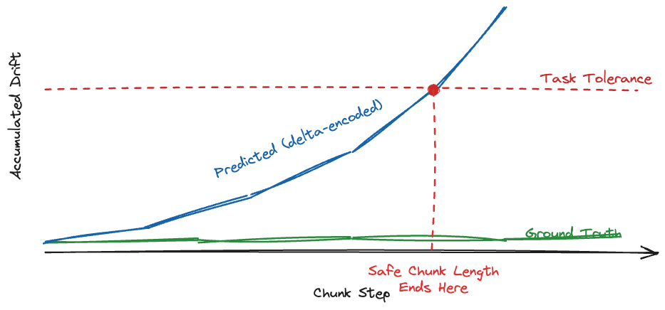
• Delta Actions: converting absolute joint angles or end-effector poses $p_t$ into frame-relative deltas $\Delta p_t = p_{t+k} - p_t$, which tends to improve numerical stability and generalization relative to training on absolute pose targets directly.

This isn't a free upgrade, though. Delta encoding pushes the cost from training onto rollout: because each predicted step is relative to the last, small per-step errors compound across a chunk in a way absolute predictions don't, and drift accumulates over the chunk horizon. It also interacts awkwardly with DAgger-style corrections, discussed earlier under upsampling—an operator correction mid-trajectory changes the reference frame the subsequent deltas are computed against, and a labeling pipeline that doesn't account for that can silently encode the correction incorrectly.

Data Augmentation Pipeline

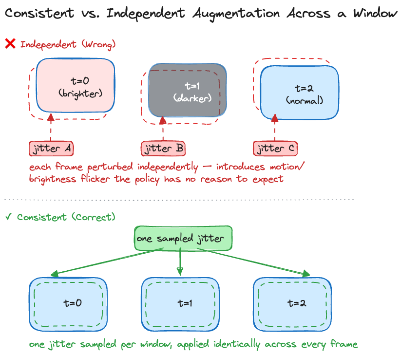
• Photometric Augmentation: dynamic brightness, compression-codec simulation, contrast jitter, and color jitter, applied consistently across every timestep within an observation horizon—jittering each frame independently would introduce spurious temporal variation the policy has no reason to expect at inference time.
• Spatial Augmentation: crop-and-resize transforms applied uniformly across multi-view camera feeds, for the same reason—independent per-view cropping would break the geometric consistency between views that the policy may be relying on.

Conditioning Dropout

Dropout, in the general sense, is one of the more underrated levers in this entire post. Every other online processor in this section perturbs how an input looks; dropout perturbs whether an input is there at all—and that distinction turns out to be doing most of the robustness work across conditioning dropout and proprioceptive noise injection, even though each is introduced as a separate technique. The underlying idea is the same one every time: any conditioning channel a model is allowed to rely on unconditionally becomes a latent single point of failure the moment that channel is degraded, delayed, or simply absent at deployment. Training with that channel occasionally missing is what forces the model to actually distribute its understanding of the task across every signal available to it, rather than quietly collapsing onto whichever one was easiest to key off of during training.

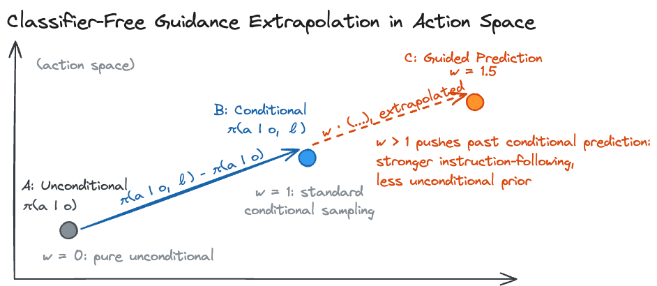
For diffusion- or flow-based action heads—increasingly the default for current VLA architectures—this general principle takes a specific, well-known form: classifier-free guidance (CFG). Randomly dropping the language instruction (or image/goal conditioning) at training time, replacing it with a null token some fraction of the time, trains the model to also produce a coherent unconditional prediction—effectively fitting two policies in one network, $p(a \mid o)$ and $p(a \mid o, \ell)$, sharing the same weights.

That unconditional branch isn't just a training-time robustness trick—it's what makes a genuinely useful inference-time control available. Once both branches exist, sampling can extrapolate along the vector between them at each denoising step:

where $\tilde{\epsilon}$ is the model's noise (or velocity) prediction rather than a directly sampled action—the extrapolation happens in score space across the iterative denoising process, not as a single linear combination of final actions, since you can't linearly interpolate the outputs of an arbitrary non-linear policy and expect the result to stay on-manifold. The guidance scale $w$ trades off instruction-following strength against the smoothness of the unconditional prior. This is the same lever text-to-image diffusion models use to make prompts "grip" harder—here it means an operator can dial up how strictly the policy adheres to a given instruction after the model is already trained, without touching the weights.

Framed this way, conditioning dropout isn't really a separate idea from proprioceptive noise injection—it's the same robustness-through-omission principle applied to language/goal conditioning specifically, which happens to come with an extra payoff (the guidance-scale knob) that adding sensor noise doesn't. It's worth calling out precisely because it's easy to implement as an afterthought—a single if random() < p: instruction = null line—while actually being one of the highest-leverage single lines in the entire online-processing stack.

Proprioceptive Noise Injection

Adding synthetic noise to joint or state inputs at training time, distinct from the sensor-health filtering discussed earlier, which removes genuinely bad proprioceptive data. This is about robustness to noise that's expected but not present in a clean offline corpus—particularly relevant for sim-to-real transfer, where simulated proprioception is often cleaner than what the real robot's encoders will report at deployment.

Weighted & Curriculum Batch Sampling

This is the section where the upsampling and mixture-ratio discussions from earlier in this post actually get realized. Filtering decides what's in the corpus; mixture weighting decides the target distribution that corpus should be trained toward; the sampler is the concrete mechanism that turns that target distribution into an actual sequence of batches. A weighted sampler drawing from persisted episode metadata—embodiment, task, success/failure—is what makes a stated mixture ratio ("40% single-arm, 25% mobile nav...") something that actually happens epoch over epoch, rather than a number that only describes the corpus's static composition.

Scale & Orchestration: Distributed Execution and Lineage

Everything described so far has been at the level of a single episode or a single batch. None of it changes conceptually at fleet scale—but running it serially, episode by episode, over 100,000+ hours of logs is simply not viable. This section covers what changes operationally, not algorithmically, once the pipeline has to run continuously against a corpus that's still growing.

Distributed Pipeline Frameworks

Most of filtering and autolabeling is embarrassingly parallel at the episode level—nothing about running a stationarity check or a VLM captioning pass on episode 40,000 depends on the result for episode 39,999. That property is exactly what distributed data-processing engines like Ray Data and Apache Spark are built to exploit: scaling filters and autolabelers out across a worker pool, operating directly on the independent Zarr/MCAP shards established in the previous post's sharding layer.

Trajectory deduplication is the explicit exception, and it's worth calling out rather than glossing over: deciding whether episode 40,000 is a near-duplicate requires comparing it against the embeddings of every other episode in its candidate cluster, which is a cross-episode reduce, not an independent per-episode map. Scheduling it like the rest of this section's embarrassingly-parallel work—hand it to a plain distributed map and walk away—gets the architecture wrong. In practice this means dedup runs as its own distinct job: build the approximate-NN index first (a distributed build step, not a map), then look up and cluster against it, which is closer to a distributed join than a distributed filter.

The independence property has a limit that matters more than the parallelism question, though. Parallelism describes how each stage is scheduled internally; it says nothing about the order stages need to run in relative to each other, and this pipeline's stages aren't strictly ordered. The feedback loops covered earlier in this post—autolabeling output retroactively re-flagging episodes back in filtering, boundary-aware stationarity filtering needing a second pass once captions exist, mixture ratios only being tunable after candidate training runs complete—aren't parallelism problems at all. They're dependency-graph problems: a given shard may need to pass through filtering, then autolabeling, then filtering again, and no amount of worker-pool scaling resolves that if the orchestration layer doesn't know a second filtering pass is owed. This is what DAG-based workflow schedulers (Airflow, Dagster, Prefect) are for, sitting a level above Ray/Spark rather than replacing them: Ray or Spark handles "run this stage across 50,000 episodes in parallel," while the DAG scheduler handles "don't start the second filtering pass on a shard until autolabeling has actually finished for it, and re-trigger mixture-ratio tuning only once a training candidate's eval run completes." Treating the whole pipeline as one flat parallel job works for a single stage; it silently drops the re-passes the earlier feedback-loop discussion depended on.

The remainder of this section is about how the worker pool underneath any of this actually gets utilized well, which turns out to look quite different depending on whether the model doing the work lives behind an API or on hardware you control.

Processing at Scale: Cloud-Based vs. On-Prem Models

Autolabeling at fleet scale generally means calling a hosted foundation model over an API (GPT-4o, Gemini Vision) or running an open-weight model on hardware you control. Both cases reduce to the same underlying discipline: identify the one hard resource ceiling that throughput cannot exceed—API requests per minute in the cloud case, GPU memory in the on-prem case—and schedule against a live measurement of that ceiling rather than a correlate of it. Idle CPU cores don't tell you anything about your API rate allocation; available RAM doesn't tell you anything about VRAM headroom. A pipeline that autoscales against the wrong proxy looks efficient right up until it hits the real ceiling and collapses into throttling or OOM failures.

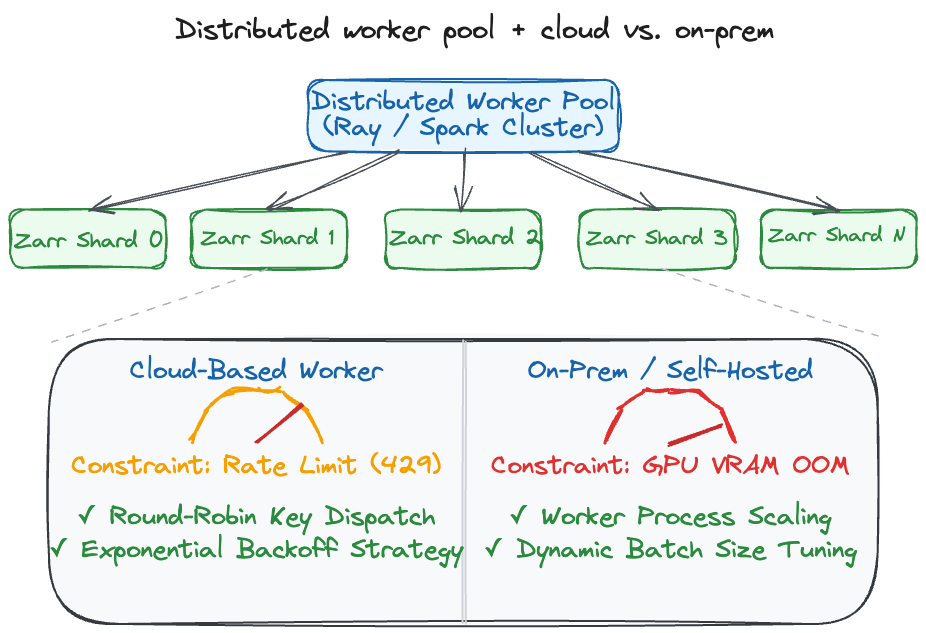
Cloud-Based (API-Backed Models): the bottleneck is the provider's rate limit, not your own compute. Spread requests across multiple keys/endpoints round-robin, back off exponentially on a rate-limit error rather than retrying immediately, and scale worker count against allocated API throughput—not against idle CPU cores, which tell you nothing about it.

On-Prem / Self-Hosted: the bottleneck inverts—no external rate limit, but a fixed, often-shared GPU pool. Schedule opportunistically against idle cluster capacity rather than holding a fixed reservation, and tune worker count and per-worker batch size jointly against available VRAM, since too many concurrent workers at too large a batch size OOMs partway through a run.

Prefetching batches applies to both: keeping several batches in flight hides whichever latency dominates—network round-trip time for cloud, disk/object-store I/O for on-prem—rather than paying it serially. It doesn't raise the ceiling; it just keeps the pipeline busy right up against it instead of idling between requests.

Incremental Mode & Checkpointing

Fleet data doesn't arrive as a single batch—it accumulates daily, from robots that are still out in the field. Re-running the full filtering-through-labeling pipeline over the entire historical corpus every time new data lands doesn't scale, and it doesn't need to: filtering and autolabeling outputs for existing episodes don't change unless the filter rules or labeler checkpoint themselves change (covered next). The practical pattern is incremental processing—running the pipeline only against newly-arrived shards, then merging the resulting manifest rows into the existing index rather than regenerating it. This applies identically whether the underlying labeling job is cloud- or on-prem-based; incremental mode is about which shards get processed, not how each one gets processed.

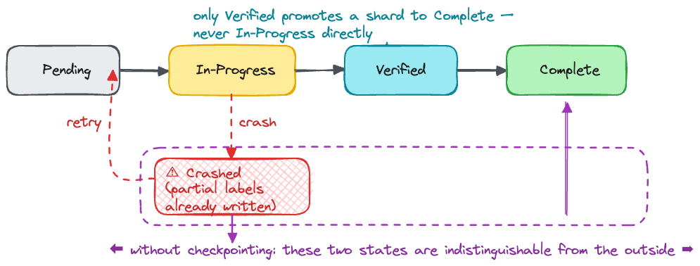
This introduces a failure mode worth guarding against explicitly, and it compounds with the rate-limit and memory-pressure concerns above: a job that fails partway through a shard—whether from a rate-limit exhaustion, an OOM, or a transient network error—shouldn't silently leave that shard half-labeled and indistinguishable from a fully-processed one. Production pipelines handle this the same way the previous post's sharded-write safety did—checkpointing progress within a job and only marking a shard's manifest entries as complete once the job finishes and is verified, so a retry after a crash or a throttling failure reprocesses cleanly rather than producing a partial, silently-corrupt label set.

Dataset Versioning & Lineage Tracking

Robot models demand strict reproducibility in a way that's easy to underinvest in until the first time it's needed urgently: when a trained policy underperforms, the first diagnostic question is almost always which data it actually trained on, and answering that requires tracking the exact combination of raw log version, filter rules, and autolabeler checkpoint that produced the dataset—not just "the dataset as of last Tuesday." This matters more, not less, once a pipeline is mixing cloud and on-prem labelers incrementally over time: a corpus assembled across months of incremental runs can easily have different shards labeled by different model versions without anyone noticing, absent an explicit record of which.

General-purpose data versioning tools are one way to make that combination reconstructable. DVC (Data Version Control) works at the git layer—it hashes large files and pipeline-stage dependencies so a corpus, a filter ruleset, and a labeler checkpoint can each be pinned to a commit. LakeFS operates one layer down, giving git-like branching and atomic commits directly on top of object storage (S3, GCS), which pairs naturally with a sharded-Zarr-on-object-storage layout specifically because a single commit can capture the shards and the manifest together, atomically.

Neither tool was purpose-built for the sharded-Zarr-plus-manifest pattern this series has been building, though, and it's worth being honest that plenty of production pipelines skip both in favor of something simpler: a version column baked directly into the manifest schema (corpus_version, filter_ruleset_commit, labeler_checkpoint), plus immutable, timestamped snapshots of the manifest file itself in object storage. That gets you most of the reproducibility guarantee below without adopting a general-purpose tool that wasn't designed around this exact storage shape. Whichever mechanism you choose, the target artifact looks the same:

Raw Corpus (v1.2) + Filtering Rules (commit e3a1) + VLM Annotator (v2.0) = Training Dataset Hash (sha256:7f9...)

Epilogue

This post traced how a raw, heterogeneous, featurized-but-unrefined robot corpus becomes something a policy can actually learn from. The path runs through deterministic and learned filters that decide what survives, mixture weighting that sets the target distribution the corpus should represent, foundation-model autolabeling that attaches the semantic signal raw sensor streams never carry, and finally the online processors that reshape all of it, on the fly, into the tensors a training step actually consumes—all of it running at fleet scale under distributed, incrementally-updated, lineage-tracked infrastructure.

Worth being honest about scale here: each of those five sections is the tip of its own iceberg. Filtering alone spans entire subfields of anomaly detection and time-series analysis; autolabeling touches everything happening in video-language modeling right now; online augmentation strategies could fill a post on their own. This one covered the shape of each problem and the patterns that recur across them—enough to build a working pipeline—not the full depth any one of them has in production at a frontier lab.

Put together with the previous two posts, that's now the complete path a single sensor reading takes: from a live DDS topic, through a chunked MCAP log, through featurization into a sharded Zarr array, through the filtering and labeling pipeline described here, and finally into a training batch a policy gradient actually flows through.

The biggest gap this post didn't resolve: this post argued for labeling generously and filtering conservatively, on the grounds that missing labels are expensive to add later and unnecessary filters are cheap to loosen. That argument assumes you can tell, after the fact, whether a given filtering or mixing decision actually helped—and this post never described how you'd know. Held-out splits are a prerequisite for answering that question, not a substitute for actually answering it, and a validated methodology for confirming that a filtering threshold, mixture ratio, or autolabeler swap improved policy performance—rather than just changed it—is conspicuously absent above.

A few other gaps worth naming directly:

• Action Tokenization & Discretization: this post assumed a continuous or diffusion-style action representation throughout the sections on action chunking and conditioning dropout, without addressing how actions become model-consumable labels in the first place—uniform-bin discretization into language-model tokens, VQ-style learned codebooks, and continuous flow/diffusion targets are genuinely different labeling decisions with different downstream implications, and the choice was never made explicit.
• Preference-Based & RL-Style Labels: every labeling method discussed is supervised and absolute—a caption, a success flag. Preference-based post-training, built on pairwise trajectory comparisons and RLHF/RLAIF-style ranking, is a structurally different labeling problem this post didn't touch.
• Sim/Real Data Blending: the mixture-ratio section treated simulation as one line in a mixture ratio without addressing how synthetic data gets validated against real-world distribution shift before it's trusted alongside real fleet data.
• PII Redaction: VLM-based autolabeling will transcribe whatever is visible in-frame—faces, badges, visible text—and detecting and redacting that before a dataset is eligible for broader use is a real pipeline stage this post skipped entirely.
• Egocentric Human-Video Pipelines: the human-video section scoped this out deliberately—3D hand pose estimation, virtual-gripper derivation, and IK-based retargeting from human video into robot action space is substantial enough to be its own post, and it remains a real gap here.

Each of those is a real system in its own right, and several are natural candidates for their own treatment later in the series. This post covered the refinement layer—if the corpus feeding a policy is noisy, imbalanced, or unlabeled, no amount of architecture cleverness downstream fully recovers from it.

Next in the series: Inside Robot Policy Serving—how trained foundation models and VLAs are deployed back onto edge hardware, covering model quantization (FP8/INT4), KV-caching for spatial transformers, real-time action chunk execution, and multi-threaded C++ inference loops that hit tight latency deadlines.

References

Brohan et al., "RT-2: Vision-Language-Action Models Transfer Web Knowledge to Robotic Control," arXiv:2307.15818, 2023.
Team et al., "Octo: An Open-Source Generalist Robot Policy," arXiv:2405.12213, 2024.
Kim et al., "OpenVLA: An Open-Source Vision-Language-Action Model," arXiv:2406.09246, 2024.
Black et al., ": A Vision-Language-Action Flow Model for General Robot Control," arXiv:2410.24164, 2024.
O'Neill et al., "Open X-Embodiment: Robotic Learning Datasets and RT-X Models," arXiv:2310.08864, 2023.
Zhao et al., "Learning Fine-Grained Bimanual Manipulation with Low-Cost Hardware (ALOHA)," arXiv:2304.13705, 2023.
LeRobot Library & Dataset Schemas, Hugging Face GitHub Repository.
Wang et al., "HumanEgo: Zero-Shot Robot Learning from Minutes of Human Egocentric Videos," arXiv:2605.24934, 2026.
Yang et al., "EgoVLA: Learning Vision-Language-Action Models from Egocentric Human Videos," arXiv:2507.12440, 2025.
Liu et al., "EgoEngine: From Egocentric Human Videos to High-Fidelity Dexterous Robot Demonstrations," arXiv:2606.12604, 2026.
Project Aria, Meta Reality Labs — Egocentric Perception Platform, projectaria.com